Analysing news broadcasted by German radio station SR2
Analysis
Topics are set and public opinion is framed by broadcasting stations. This project wants to analyze the daily news broadcasted by German radio station SR2.
Show the code
# Setup# Load pckgslibrary(knitr)library(tidytext)library(tidyverse)library(RColorBrewer)library(wordcloud)# Load datafolder <-"../../../3_SR2 News Mining/data"files <-list.files(folder, pattern =".Rdata", full.names =TRUE)loaded_data <-vector("list")for (file in files) {load(file) loaded_data[[file]] <- news # Assuming the data frames are named "news"}news_raw <-map2(loaded_data, names(loaded_data), ~mutate(.x, source_file = .y)) %>%map(bind_rows) %>%list_rbind() %>%as_tibble()
Overview
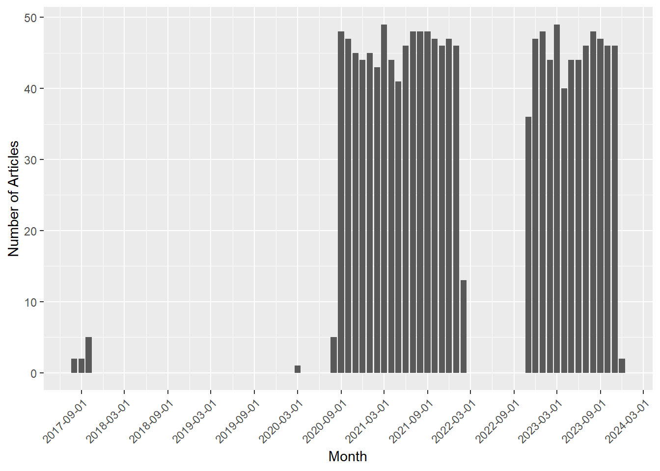
The data collected from the webpage goes from 2017-08-31 to 2023-12-01.
If we have a closer look on the URLs, we can see that every article has an identification number associated which comes after the id= parameter at a similar position for each URL.
By clicking on a link, we also note, that many pages have gone offline already. Because we have scraped the page over time, we can now observe that a few articles have modified their news message afterwards. However, these were only minor changes.
“Planer” der IS-Miliz in Afghanistan im Visier - USA fliegen Drohnenangriff / Trotz Terrorwarnung - Tausende Menschen versuchen Kabul zu verlassen und das Interview der Woche mit Jens Spahn, Bundesgesundheitsminister
“Planer” der IS-Miliz in Afghanistan im Visier - USA fliegen Drohnenangriff / Trotz Terrorwarnung - Tausende Menschen versuchen Kabul zu verlassen / Interview der Woche mit Jens Spahn, Bundesgesundheitsminister (CDU)
22080
Gewagtes Schutzversprechen - Bisher nur 138 deutsche Ortskräfte ausgeflogen / Nach britischem Abzug - Kritik an Regierung Johnson / Die Preise steigen - wirklich nur vorübergehend? - Hohe Inflationsrate befürchtet
Gewagtes Schutzversprechen - Bisher nur 138 deutsche Ortskräfte ausgeflogen / Nach britischem Abzug - Kritik an Regierung Johnson / Die Preise steigen - wirklich nur vorübergehend? Hohe Inflationsrate befürchtet
22586
Kommentar zum Ende der Sondierungsgespräche / Ab heute Kita-Lockerungen: Fluch und Segen / Pandora Papers: Warum funktionieren Briefkastenfirmen trotz Regulierung? / EU-Parlament verurteilt Belarus / Abholzung in Kongo
Kommentar zum Ende der Sondierungsgespräche / Ab heute Kita-Lockerungen - Fluch und Segen / Pandora Papers - Warum funktionieren Briefkastenfirmen trotz Regulierung? / EU-Parlament verurteilt Belarus / Abholzung in Kongo
Let’s examine the time frame covered by the articles.
Show the code
# Articles by monthnews_distinct %>%count(Month =floor_date(Datum, "month"),name ="Number of Articles") %>%ggplot(aes(x = Month, y =`Number of Articles`)) +geom_col() +scale_x_date(date_breaks ="6 months") +theme(axis.text.x =element_text(angle =45, vjust =1, hjust =1))
Our data shows two time periods that are uncovered. The first is before August 2020. Unfortunately, SR2 seems to have deleted their data or they simply did not upload their editions consequently before that date. Therefore, to not bias our analysis, the 80 articles from before August 2020 are deleted (listwise deletion, since these are just a few cases). Moreover, we identify a significant gap in information between February and October 2022. You see, behind this code there is a human and humans aren’t robots. Sometimes life throws in its own surprises and a unique blend of personal events distracted me from continuing this analysis. But I’m back in action now!😊
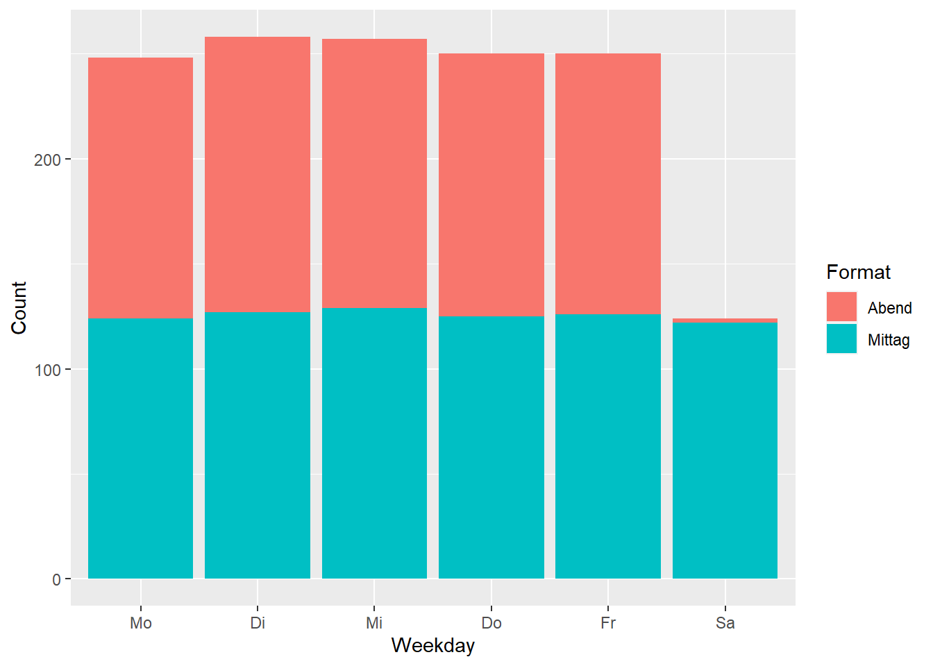
We then observe, while Bilanz am Abend is published on weekdays, Bilanz am Mittag also appears on Saturdays. Sunday is a holiday.
Show the code
# Articles by day of weeknews_filtered %>%count(Format,Weekday =wday(Datum, locale ="German", label =TRUE),name ="Count") %>%ggplot(aes(x = Weekday, y = Count, fill = Format)) +geom_col()
Authors
When focusing on the narrators, it is interesting to note how the SR webpage content managers do not know the names of their colleagues. Or what is the reasons of that many different spellings of the same name?
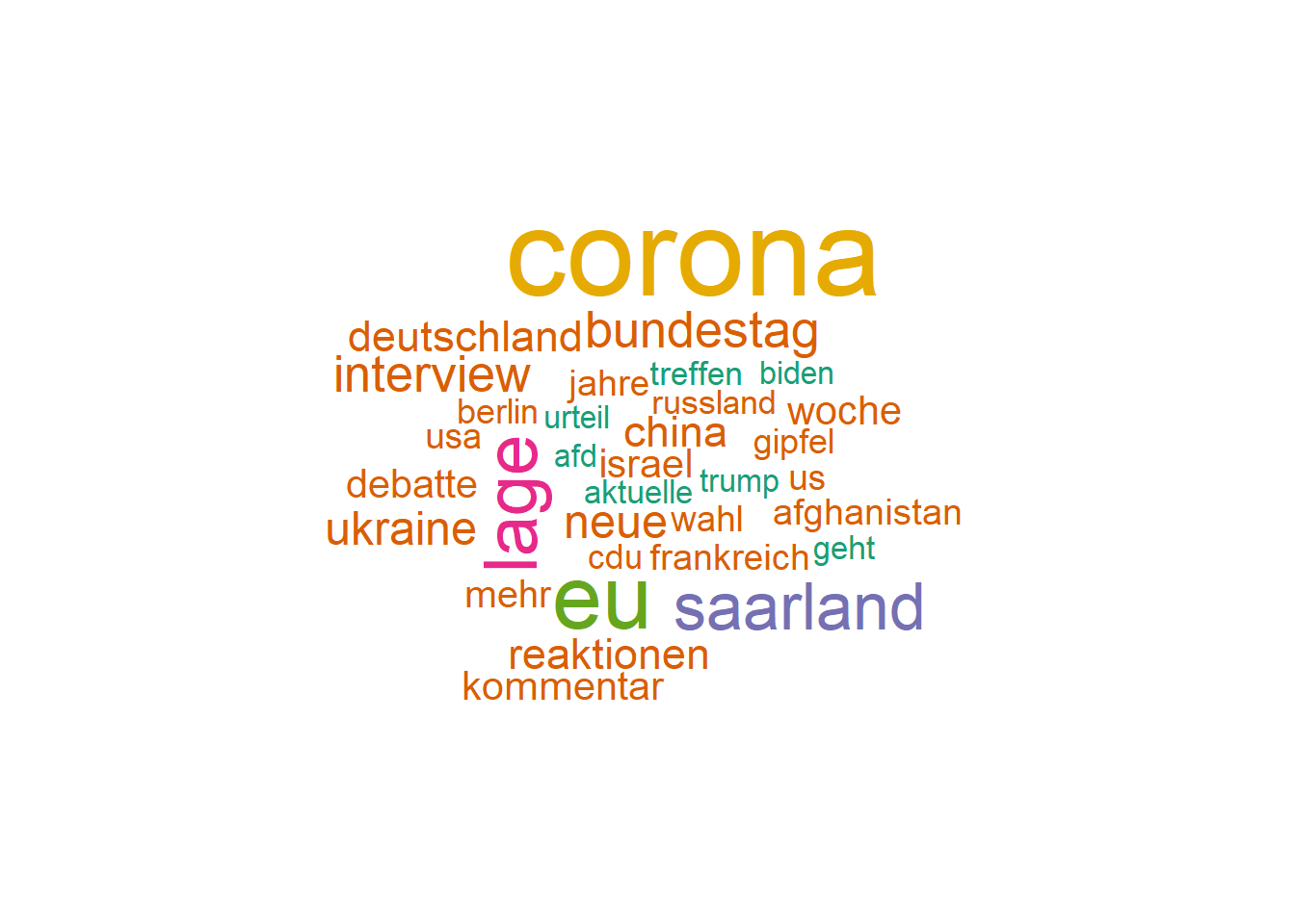
We see, Corona clearly dominated the news and also EU related topics were discussed. Since SR2 is a regional broadcasting station, it’s no surprise that we also observe the keyword Saarland. If we sum up all US related keywords that show up (Biden, Trump, USA, US) we notice it is another very dominant topic.
Show the code
# Frecuency US related wordsusa_keywords <-c("biden", "trump", "usa", "us")news_unnested %>%mutate(Word =ifelse(Wort %in% usa_keywords,"US_keywords_summary", Wort)) %>%count(Word, name ="Count", sort =TRUE) %>%head(3) %>%kable()
Word
Count
corona
384
eu
263
US_keywords_summary
261
It is also interesting to observe the distribution of these keywords within the week.
Corona and the Ukraine dominate news during the week, indicating perhaps an avoidance of such pressing topics on weekends. Saturdays seem reserved for more background information, as implied by the prominence of the word “interview”. US-related topics persist from Monday to Saturday, and I wonder why a similar pattern does not seem to hold for other countries, such as China. Regional messages concerning the Bundestag (the German Parliament), Saarland or the EU take center stage during weekdays.
Keywords over time
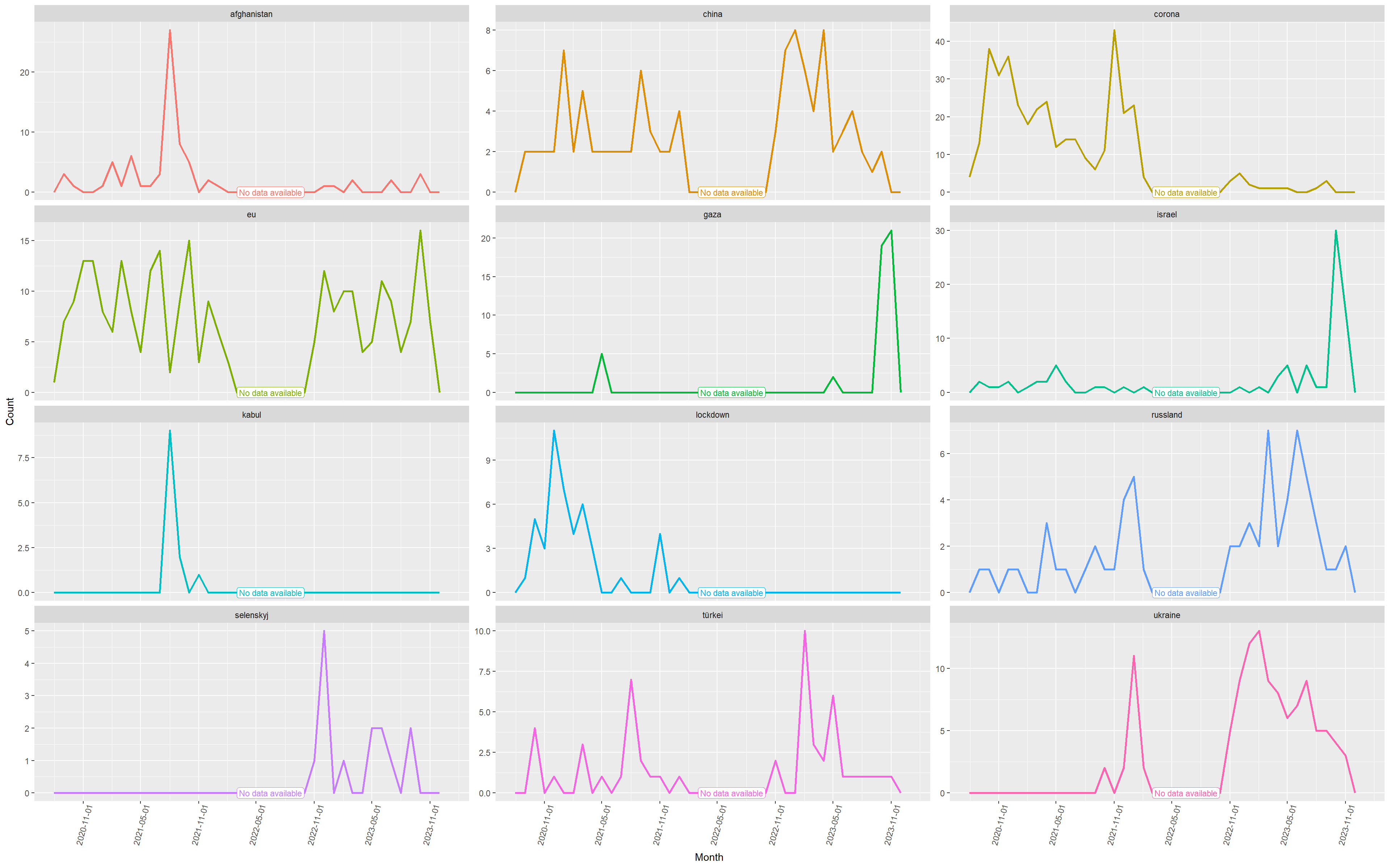
Let’s visualize the changing patterns of specific keyword appearances over time.
Show the code
# Select keywordskeywords <-c("lockdown", "corona", "afghanistan", "kabul", "ukraine", "russland", "gaza", "israel", "china", "türkei", "eu", "selenskyj")# Selected keywords over timenews_unnested %>%count(Wort, Month =floor_date(Datum, "month"), name ="Count") %>%filter(Wort %in% keywords) %>%# If keyword does not appear in certain month, insert row with explicit 0complete(Month =seq(from =floor_date(min(news_unnested$Datum), "month"),to =max(news_unnested$Datum),by ="month"), Wort,fill =list(Count =0)) %>%ggplot(aes(x = Month, y = Count, color = Wort)) +geom_line(linewidth =1) +geom_label(aes(label ="No data available", x =as_date("2022-06-15"), y =0), size =3, label.padding =unit(.15, "lines")) +facet_wrap(~ Wort, ncol =3, scales ="free_y") +scale_x_date(breaks ="6 month", limits =c(NA_Date_, floor_date(today() -months(1), "month"))) +theme(legend.position ="none",axis.text.x =element_text(angle =75, vjust =0.58))
It’s interesting to see how news themes develop in the course of time. Gaza and Israel have a peak since October 2023, but note that Israel appears twice as often as Gaza. Accordingly, the Ukraine is every day of fewer importance and maybe soon to disappear, although the war is going on? Corona and lockdown are not present anymore, however at the end of each year it feels like Corona celebrates its comeback in the news.
NB: This project was a work in progress from September 2020 until December 2023. Moving forward, I won’t be sending regular updates. However, I am considering to use this experience to extend it to another media website, driving it towards a more professional level and maybe a broader audience. More to come…