---
freeze: true
title: "Cruise Tourism Is More Extreme Than You Think"
author: "Me"
date: "2026-04-01"
categories: [Data Analytics, Social Processes]
format:
html:
toc: true
code-tools: true
execute:
warning: false
echo: false
fig-width: 10
fig-asp: 0.618
out-width: "100%"
fig-align: center
---
```{r}
#| label: setup
# Load libraries for functions to work
library(httr2)
library(tidyverse)
library(scales)
library(knitr)
library(kableExtra)
options(scipen = 999)
linecolor <- c("darkorange", "cadetblue", "black")
plot_style <- theme_minimal() +
theme(plot.title = element_text(hjust = 0.5, size = 20, face = "bold"),
panel.grid.minor.x = element_blank(),
strip.text = element_text(size = 20, face = "bold"),
axis.text = element_text(size = 14),
axis.text.x = element_text(angle = 45),
axis.title = element_text(size = 14),
legend.text = element_text(size = 14),
legend.title = element_text(size = 14))
```
### What’s in here?
Each year, thousands of cruise passengers arrive in the beautiful Spanish city of La Coruña. But who is actually coming and how concentrated is this?
This analysis breaks down the patterns behind cruise arrivals using data since 2024 scraped from the official website of [Autoridad Portuaria de A Coruña](https://www.puertocoruna.com){target="_blank"}.
::: {.callout-note}
This article was first published on `2026-04-01` and last updated on ``r Sys.Date()``.
:::
```{r}
#| label: scrape and save data
#| eval: false
# Create URL List
months <- seq(as.Date("2024-01-01"), to = today(), by = "month")
url_list <- sprintf(
"https://www.puertocoruna.com/o/api/escalas/publicas/%02d/%d",
as.integer(format(months, "%m")),
as.integer(format(months, "%Y"))
)
# Create function to fetch data
fetch_data <- function(url) {
resp <- request(url) %>% req_perform()
raw_data <- resp %>% resp_body_json()
}
raw_data_list <- map(url_list, fetch_data) %>%
# merge into one single list
flatten()
data <- raw_data_list %>%
map_dfr(as_tibble)
# Save data
save(data, file = paste0("data/cruises_", today(), ".RData"))
```
```{r}
#| label: load data
file_name <- "data/cruises_2026-06-03.RData"
load(file_name)
```
```{r}
#| label: demographics
# Additional data
# According to www.laopinioncoruna.es/coruna/2026/02/17/cambio-tendencia-coruna-casco-urbano-126903205.html
# and www.lavozdegalicia.es/noticia/coruna/coruna/2025/12/04/area-coruna-crece-superar-461000-residentes/00031764873579905163921.htm
visma_2025 <- 3208
elvina_2025 <- 17479
san_cristobal_2025 <- 8747
oza_2025 <- 7027
coruna_nuc_2025 <- 214816
coruna_m_2025 <- visma_2025 + elvina_2025 + san_cristobal_2025 + oza_2025 + coruna_nuc_2025
```
```{r}
#| label: data manipulation
# Solve port name inconsistencies
port_map <- tribble(
~from, ~to,
"ARRECIFE DE LANZAROTE", "ARRECIFE",
"BREMENHAVEN", "BREMERHAVEN",
"CASA BLANCA", "CASABLANCA",
"CÁDIZ", "CADIZ",
"CHERBOURGO", "CHERBOURG",
"DUBLÍN", "DUBLIN",
"DUN LAOGHAIRE", "DUBLIN",
"FUNCHAL", "MADEIRA",
"GETXO", "BILBAO",
"GUERNSEY", "ST PETER PORT",
"HAMBURGO", "HAMBURG",
"HAMILTON (BERM.)", "HAMILTON(BERMUDAS)",
"LEVERDON", "LE VERDON (FR.)",
"LE VERDON (FRA.)", "LE VERDON (FR.)",
"PAL. DE MALLORCA", "PALMA DE MALLORCA",
"PONTADELGADA", "PONTA DELGADA",
"PORTLAND(UK)", "PORTLAND",
"PORTSMOUTH (UK)", "PORTSMOUTH",
"PORT MEDOC (FR)", "LE VERDON (FR.)",
"ST. MALÓ", "ST MALÓ",
"ST, MALÓ", "ST MALÓ",
"ST. PETER PORT", "ST PETER PORT",
"ST PETERPORT", "ST PETER PORT",
"ST.PETER PORT", "ST PETER PORT",
"S. CRUZ TENERIFE", "TENERIFE",
"ST. CRUZ TENERIFE", "TENERIFE",
"TILBURY", "LONDON",
"TILBURY (UK)", "LONDON",
"VILLAGAARCÍA", "VILLAGARCIA",
"VILLAGARCÍA", "VILLAGARCIA",
"ZEEBRUGGE BÉLGICA", "ZEEBRUGGE",
"TBC", "N/A"
)
data_clean <- data %>%
# Organize date time columns
mutate(
eta_dt = ymd_hms(eta, tz = "UTC"),
eta_date = date(eta_dt),
eta_time = format(eta_dt, "%H:%M:%S"),
etd_dt = ymd_hms(etd, tz = "UTC"),
etd_date = date(etd_dt),
etd_time = format(etd_dt, "%H:%M:%S")
) %>%
# Clean up port names
mutate(
puertoAnterior_clean = puertoAnterior %>%
str_trim() %>% # remove trailing spaces
str_to_upper() %>% # standardize case
str_replace_all("\\s+", " "), # normalize spaces
puertoPosterior_clean = puertoPosterior %>%
str_trim() %>% # remove trailing spaces
str_to_upper() %>% # standardize case
str_replace_all("\\s+", " ") %>% # normalize spaces
str_remove("^[^A-Za-z]+") # remove leading junk
) %>%
mutate(
puertoAnterior_clean = replace_values(puertoAnterior_clean, from = port_map$from, to = port_map$to),
puertoPosterior_clean = replace_values(puertoPosterior_clean, from = port_map$from, to = port_map$to)
) %>%
# Filter data to only consider data until the last full month
filter(eta_date < floor_date(today(), unit = "months"))
# Enrich data with Country information
get_port_country <- function(port) {
case_when(
port %in% c(
"ALICANTE", "ARRECIFE", "BILBAO", "CADIZ", "CEE", "GIJÓN", "ISLAS CIES", "MALAGA",
"PALMA DE MALLORCA", "SAN SEBASTIAN", "SANTANDER", "SEVILLA", "ST. CRUZ DE LA PALMA",
"TENERIFE", "VALENCIA", "VIGO", "VILLAGARCIA", "PORTOSIN (MUROS)"
) ~ "Spain",
port %in% c(
"BRISTOL", "BELFAST", "DOVER", "FALMOUTH", "LIVERPOOL", "LONDON", "NEWCASTLE",
"PLYMOUTH", "PORTLAND", "PORTSMOUTH", "SOUTHAMPTON", "TRESCO (U.K)"
) ~ "United Kingdom",
port %in% c(
"BANTRY (IRLANDA)", "DUBLIN", "GLENGARRIF (IRL)"
) ~ "Ireland",
port %in% c(
"BURDEOS", "CHERBOURG", "CONCARNEAU", "HONFLEUR", "LA ROCHELE", "LE HAVRE",
"LE VERDON (FR.)", "NANTES", "ST. JUAN DE LUZ", "ST MALÓ"
) ~ "France",
port %in% c(
"LEIXOES", "LISBOA", "MADEIRA", "PONTA DELGADA", "PORTIMAO", "PRAIA DA VICTORIA", "VELAS (AZORES)"
) ~ "Portugal",
port %in% c(
"BREMERHAVEN","HAMBURG"
) ~ "Germany",
port %in% c(
"CAGLIARI"
) ~ "Italy",
port %in% c(
"ROTHERDAM"
) ~ "Netherlands",
port %in% c(
"CASABLANCA"
) ~ "Morocco",
port %in% c(
"ZEEBRUGGE"
) ~ "Belgium",
port %in% c(
"GIBRALTAR"
) ~ "Gibraltar",
port %in% c(
"ST PETER PORT"
) ~ "Guernsey",
port %in% c(
"PUERTO CAÑAVERAL ( FLORIDA)"
) ~ "United States",
port %in% c(
"ST JOHN`S ANTIGUA"
) ~ "Antigua and Barbuda",
port %in% c(
"HAMILTON(BERMUDAS)"
) ~ "Bermuda"
)
}
# The "data_clean_enriched" dataset is not used in this file!
data_clean_enriched <- data_clean %>%
mutate(
puertoAnterior_country = get_port_country(puertoAnterior_clean),
puertoPosterior_country = get_port_country(puertoPosterior_clean)
)
```
### Analysis
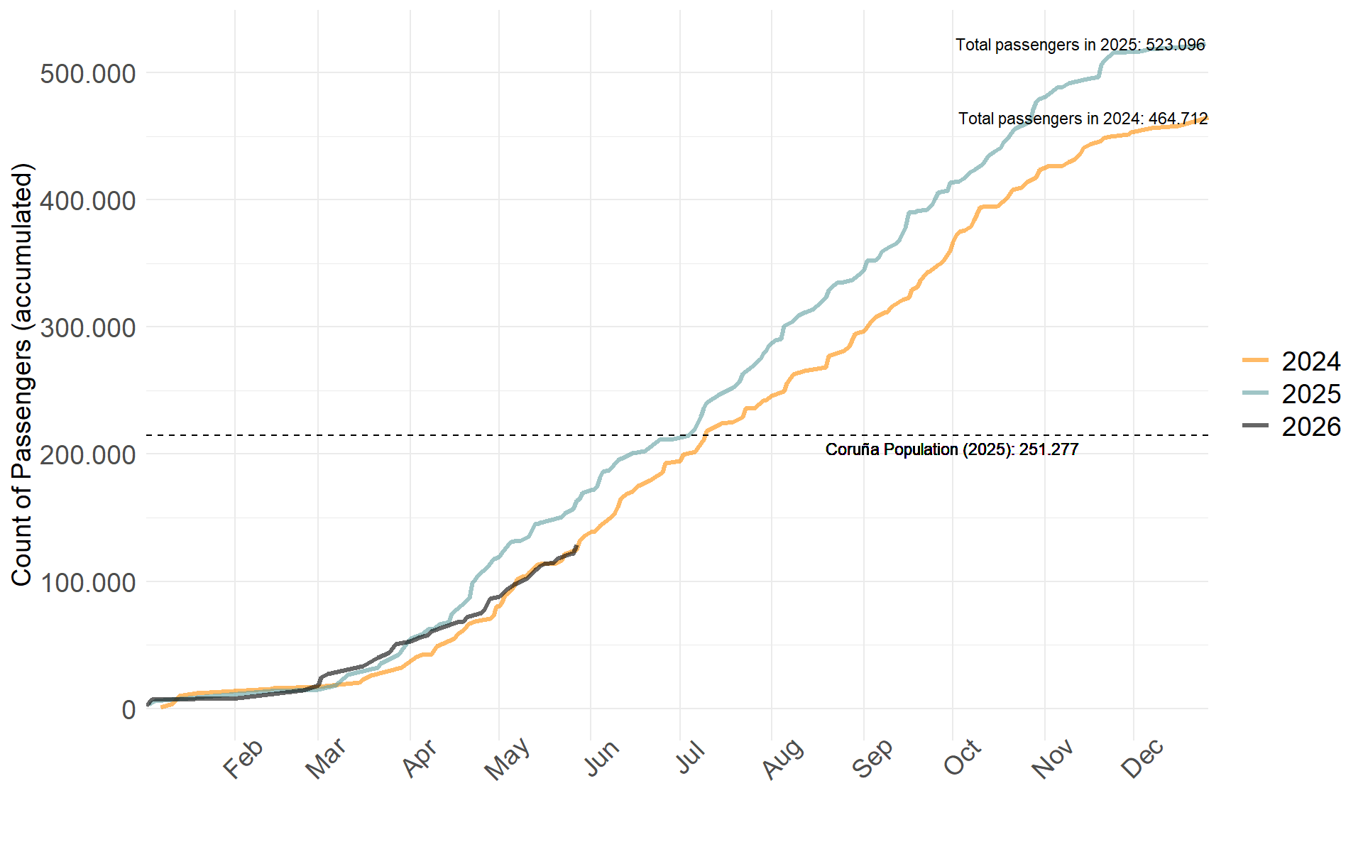
La Coruña welcomes around 500.000 visitors by sea every year. This is two times the equivalent of its entire population. Let's check if numbers are increasing in 2026.
```{r}
#| label: total pax per year
plot_data <- data_clean %>%
group_by(year = year(eta_date), eta_date) %>%
summarise(pax_per_day = sum(paxEstimados)) %>% # ungroups the last group (per day group); so it's still grouped by year
mutate(
pax_per_day_cum = cumsum(pax_per_day),
date_dummy = as.Date(paste0("2099-", format(eta_date, "%m-%d"))) # same year for all
)
# Last point per year
labels_data <- plot_data %>%
group_by(year) %>%
slice_max(date_dummy, n = 1, with_ties = FALSE) %>%
ungroup() %>%
filter(year != '2026')
plot_data %>%
ggplot(aes(x = date_dummy, y = pax_per_day_cum, color = factor(year), group = year)) +
geom_line(linewidth = 1.2, alpha = 0.6) +
geom_hline(yintercept = coruna_nuc_2025, linetype = "dashed") +
geom_text(
data = labels_data,
aes(label = paste0("Total passengers in ", year, ": ", comma(pax_per_day_cum, big.mark = ".", decimal.mark = ","))),
hjust = 1, color = "black", size = 3) +
geom_text(
x = as.Date("2099-10-01"),
y = coruna_nuc_2025,
label = paste0("Coruña Population (2025): ", comma(coruna_m_2025, big.mark = ".", decimal.mark = ",")), vjust = 1.5, color = "black", size = 3) +
scale_x_date(date_breaks = "1 months", date_labels = "%b", expand = c(0, 0)) + # use expand to avoid that ggplot extends the x-axis until Jan
scale_y_continuous(labels = label_number(big.mark = ".", decimal.mark = ",")) +
scale_color_manual(values = linecolor) +
labs(
x = "",
y = "Count of Passengers (accumulated)",
color = "",
# title = "Total Cruise Passengers"
) +
plot_style
```
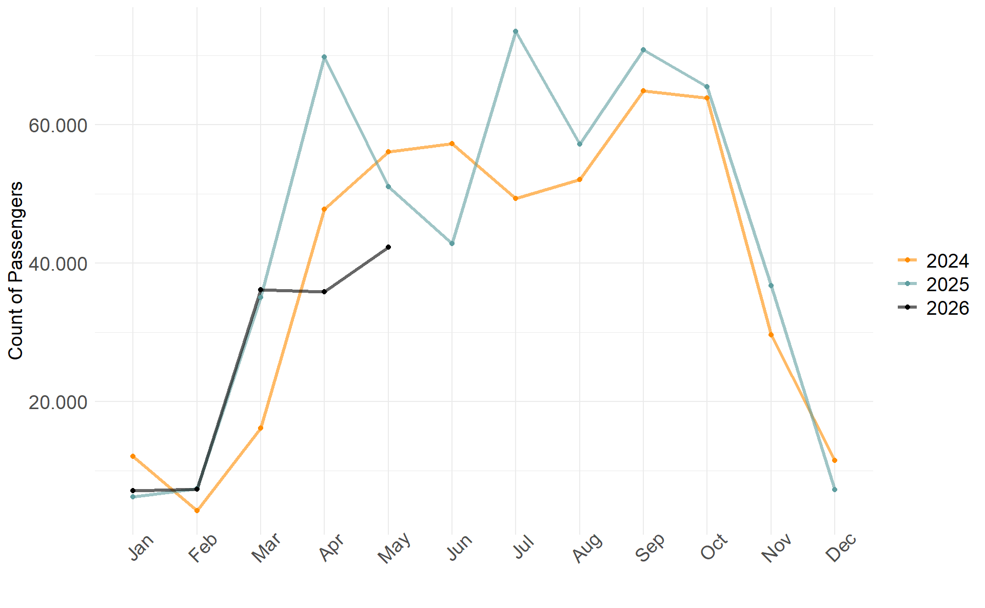
But cruise tourism comes in waves. After a quiet winter, activity accelerates sharply from spring onwards and lasts through summer and early autumn. In the last years, the pattern has remained consistent: a concentrated surge between April and October, when the vast majority of passengers typically arrives.
However, in 2026, the city enjoyed a relatively calm April and May. Are inflation, geopolitics or recent health incidents on cruise ships starting to reshape demand?
```{r}
#| label: seasonality
data_clean %>%
mutate(
year = year(eta_date),
month = month(eta_date, label = TRUE, abbr = TRUE)
) %>%
group_by(year, month) %>%
summarise(pax_per_month = sum(paxEstimados)) %>%
ggplot(aes(x = month, y = pax_per_month, group = year, color = factor(year))) +
geom_line(linewidth = 1.2, alpha = 0.6) +
geom_point() +
scale_y_continuous(labels = label_number(big.mark = ".", decimal.mark = ",")) +
scale_color_manual(values = linecolor) +
labs(
x = "",
y = "Count of Passengers",
color = "",
# title = "Monthly Cruise Passengers"
) +
plot_style
```
Most days pass unnoticed. But last year on September 16th and April 22nd, La Coruña experienced something very different: nearly 12.000 passengers arriving at once. In just a few hours, the city absorbed a surge of visitors equivalent to a small town.
Here are the five busiest days since 2024.
```{r}
#| label: pax per day
data_clean %>%
group_by(Date = format(eta_date, "%A, %B %e, %Y")) %>%
summarise(`Total Passengers` = sum(paxEstimados)) %>%
arrange(-`Total Passengers`) %>%
head(5) %>%
kable(format.args = list(big.mark = ".", decimal.mark = ","), row.names = TRUE)
```
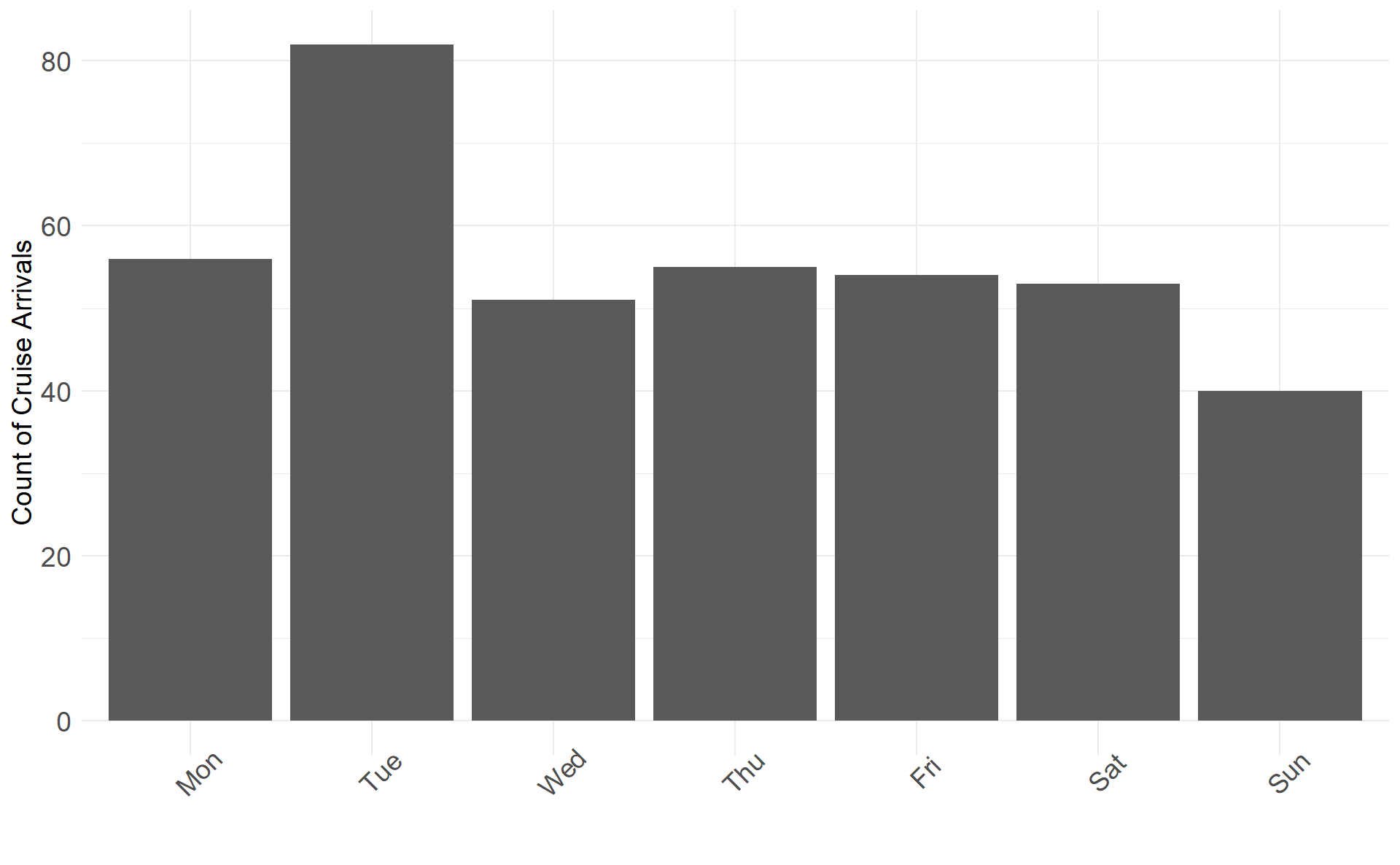
<br /> Peak days tend to cluster around Tuesdays. Overnight stays are rare, only a handful of ships remain in port meaning visitors arrive and depart within the same day. The chart below shows this clear weekday pattern.
```{r}
#| label: weekdays
data_clean %>%
count(weekdays = wday(eta_date, label = TRUE, abbr = TRUE, week_start = 1)) %>%
ggplot(aes(x = weekdays, y = n)) +
geom_col() +
labs(
# title = "Count of Cruise Arrivals per Day of Week",
x = "",
y = "Count of Cruise Arrivals"
) +
plot_style +
theme(legend.position = "none")
```
If you find yourself in the old town on a cruise day, it’s all about timing. The busiest window runs roughly from 8:00h to 17:00h. The table below shows when ships typically arrive and depart.
::: panel-tabset
#### Most Frequent Arrival Times
```{r}
#| label: arrival times
data_clean %>%
count(`Time` = eta_time, name = "Count of Cruise Arrivals", sort = T) %>%
head(5) %>%
kable(row.names = TRUE)
```
#### Most Frequent Departure Times
```{r}
#| label: departure times
data_clean %>%
count(`Time` = etd_time, name = "Count of Cruise Departures", sort = T) %>%
head(5) %>%
kable(row.names = TRUE)
```
:::
So far, we have seen how many tourists come and when. But who is actually sending all these visitors?
One port stands out: Southampton. Since 2024, more than 380.000 passengers have arrived from there alone. In fact, the most frequent route links Southampton, La Coruña and Palma de Mallorca — placing the city on a major cruise corridor.
::: panel-tabset
#### Where do they come from?
```{r}
#| label: origin
data_clean %>%
mutate(
puertoAnterior_clean = str_to_title(puertoAnterior_clean),
puertoPosterior_clean = str_to_title(puertoPosterior_clean)
) %>%
group_by(puertoAnterior_clean) %>%
summarise(pax = sum(paxEstimados), n = n()) %>%
arrange(-pax) %>%
head(5) %>%
kable(
format.args = list(big.mark = ".", decimal.mark = ","),
col.names = c("Origin Port", "Total Passengers", "Count of Cruises"),
row.names = TRUE)
```
#### Where do they go next?
```{r}
#| label: destination
data_clean %>%
mutate(
puertoAnterior_clean = str_to_title(puertoAnterior_clean),
puertoPosterior_clean = str_to_title(puertoPosterior_clean)
) %>%
group_by(puertoPosterior_clean) %>%
summarise(pax = sum(paxEstimados), n = n()) %>%
arrange(-pax) %>%
head(5) %>%
kable(
format.args = list(big.mark = ".", decimal.mark = ","),
col.names = c("Destination Port", "Total Passengers", "Count of Cruises"),
row.names = TRUE)
```
#### Full Route
```{r}
#| label: full route
data_clean %>%
mutate(
puertoAnterior_clean = str_to_title(puertoAnterior_clean),
puertoPosterior_clean = str_to_title(puertoPosterior_clean)
) %>%
group_by(puertoAnterior_clean, puertoPosterior_clean) %>%
summarise(pax = sum(paxEstimados), n = n()) %>%
arrange(-pax) %>%
head(5) %>%
kable(
format.args = list(big.mark = ".", decimal.mark = ","),
col.names = c("Origin Port", "Destination Port", "Total Passengers", "Count of Cruises"),
row.names = TRUE)
```
:::
Most ships dock at the city port of Trasatlanticos which is the main gateway into the city. The breakdown below shows how traffic is distributed across terminals.
```{r}
#| label: city port specification
data_clean %>%
mutate(nombreMuelle = str_to_title(nombreMuelle)) %>%
mutate(nombreMuelle = if_else(nombreMuelle == "Pendiente Confirmación", "Pendiente Confirmación*", nombreMuelle)) %>%
group_by(nombreMuelle) %>%
summarise(pax_sum = sum(paxEstimados)) %>%
arrange(-pax_sum) %>%
kable(
format.args = list(big.mark = ".", decimal.mark = ","),
col.names = c("City Port", "Total Passengers"),
row.names = TRUE)
```
*Note: many 2024 arrivals were recorded without a confirmed berth only indicating "Pendiente Confirmación".*
<br /> The largest ship by length was the *Anthem of the Seas*, measuring 347 meters. In terms of capacity, the Arvia stands out, carrying up to 6.685 passengers.
To put this into perspective, lining up all cruise ships arriving in the year 2025 would create a chain over 48 kilometers long — as long as the route from La Coruña to Ferrol.
::: panel-tabset
#### Largest Cruises (length)
```{r}
#| label: longest cruises
data_clean %>%
distinct(nombreBuque = str_to_title(nombreBuque), eslora) %>%
arrange(-eslora) %>%
head(5) %>%
kable(col.names = c("Cruise Name", "Length (m)"),
row.names = TRUE)
```
#### Largest Cruises (passengers)
```{r}
#| label: largest cruise
data_clean %>%
distinct(nombreBuque = str_to_title(nombreBuque), paxEstimados) %>%
arrange(-paxEstimados) %>%
head(5) %>%
kable(
format.args = list(big.mark = ".", decimal.mark = ","),
col.names = c("Cruise Name", "Total Passengers"),
row.names = TRUE)
```
*Note: the Arvia appears twice in this table, reflecting an increase in capacity between the 2024 and 2025 seasons.*
:::
### What does it all mean for us, the residents?
For a few hours, on a handful of days, the city fills up fast. Streets get busier, queues grow longer and the pace changes. For us, the residents, this translates into crowded streets, shifting daily rhythms and a city that briefly operates at a different scale.
This creates both opportunity and pressure, making timing and distribution key levers for better city management.
### References
- Data was collected from the official website of [Autoridad Portuaria de A Coruña](https://www.puertocoruna.com){target="_blank"} through a web scraping algorithm and analysed using the R programming language.
- Check out my [GitHub repository](https://github.com/dani-f/Cruise-Tourism){target="_blank"} to see how the data was scraped, cleaned and analysed and how this report was compiled.